Reinforcement Learning for Flight Control Systems

This repository implements deep reinforcement learning to train flight control systems (FCS) for a fixed-wing aircraft. The project includes a simulator, a web-app for testing the simulator using keyboard inputs, and a complete environment for training RL agents. This implemented environment is used to train agents using the Proximal Policy Optimization (PPO) algorithm from the Stable Baselines3 library to follow specific flight paths given by waypoints.

Requirements and Installation

Clone the repository:

git clone <repository-url>
cd rl-fcs

To set up the environment, you need to install the required python packages. You can do this using pip:

pip install -r requirements.txt

For Weights & Biases (WandB) integration, you need to login to your WandB account or uncomment the corresponding lines in the training script for offline mode. If using online mode, you also need to create a new project on WandB named rl-fcs and set the entity to your username or team name in training/waypoint/train_waypoint_control.py.

wandb login

To use the web-app, navigate to the web-app directory and install node if you haven’t already. Then, install the necessary npm packages following the instructions in the web-app/README.md file. This are the main steps:

cd simulator_webapp
npm install

To run the web-app, use:

npm run dev

Simulator

In order to have a Flight Dynamics Model (FDM) for the aircraft and implement the environment, a simple simulator was developed in Python using the linearized equations of motion from a reference condition and integrating them using a Runge-Kutta 4th order method. The complete steps to derive the equations can be found in Chapter 14 of the book [1] and Ronge Kutta integration in page 905 of [2].

The Euler equations of motion result of applying the linear momentum theorem and the angular momentum theorem to a rigid body in flight. Then using the Coriolis theorem to express the time derivative from an inertial frame to a body frame, assuming the airplane is symmetric so only $I_{x}, I_{y}, I_{z}, J_{xz}$ are non-zero, and finally separating the forces and moments into thrust, aerodynamic and weight components, we obtain the following equations in body axes:

$$\vec{F} = \frac{\mathrm{d}(m \vec{V})}{\mathrm{d} t} \Rightarrow \begin{cases} -m g \sin \theta + F_{T x} + F_{A x} = m(\dot{u} - r v + q w) \\ m g \cos \theta \sin \phi + F_{T y} + F_{A y} = m(\dot{v} + r u - p w) \\ m g \cos \theta \cos \phi + F_{T z} + F_{A z} = m(\dot{w} - q u + p v) \end{cases}$$ $$\vec{G} = \frac{\mathrm{d}(I \vec{\omega})}{\mathrm{d} t} \Rightarrow \begin{cases} L_T + L_A = I_x \dot{p} - J_{x z} \dot{r} + (I_z - I_y) q r - J_{x z} p q \\ M_T + M_A = I_y \dot{q} - (I_z - I_x) p r + J_{x z} (p^2 - r^2) \\ N_T + N_A = I_z \dot{r} - J_{x z} \dot{p} - (I_x - I_y) p q + J_{x z} q r \end{cases}$$

In addition, the kinematic angular equations are obtained projecting the euler angular rates from each Tait-Bryan rotation axis to the body frame:

$$\begin{array}{l} p = \dot{\phi} - \dot{\psi} \sin \theta \\ q = \dot{\theta} \cos \phi + \dot{\psi} \cos \theta \sin \phi \\ r = -\dot{\theta} \sin \phi + \dot{\psi} \cos \theta \cos \phi \end{array}$$

Finally, the kinematic translational equations are obtained projecting the body frame velocities to the inertial frame:

$$\begin{cases} \dot{x}_e &= (\cos \theta \cos \psi) u+(\sin \phi \sin \theta \cos \psi-\cos \phi \sin \psi) v+(\cos \phi \sin \theta \cos \psi+\sin \phi \sin \psi) w \\ \dot{y}_e &= (\cos \theta \sin \psi) u+(\sin \phi \sin \theta \sin \psi+\cos \phi \cos \psi) v+(\cos \phi \sin \theta \sin \psi-\sin \phi \cos \psi) w \\ \dot{z}_e &= -\sin \theta u+\sin \phi \cos \theta v+\cos \phi \cos \theta w \end{cases}$$

This equations are then linearized around a reference condition which is a steady, straight, symmetric, wing-level flight asumming stability axis ($\alpha_s=0$) and $\psi_s=0$:

$$\begin{aligned} \dot{u}_s=\dot{v}_s=\dot{w}_s=0 \\ p_s=q_s=r_s=0 \\ \alpha_s=\beta_s=0 \\ \phi_s= \theta_s = \psi_s=0 \\ \end{aligned}$$

From this reference condition, a perturbation is applied to each state variable, for example $u=u_s+\Delta u$, and after neglecting second order terms, the linearized equations of motion are obtained:

$$\begin{cases} -m g \cos \theta_s \Delta \theta+\Delta F_{T x}+\Delta F_{A x} &=m \Delta \dot{u} \\ m g \cos \theta_s \Delta \phi+\Delta F_{T y}+\Delta F_{A y} &=m\left(\Delta \dot{v}+u_s \Delta r\right) \\ -m g \sin \theta_s \Delta \theta+\Delta F_{T z}+\Delta F_{A z} &=m\left(\Delta \dot{w}-u_s \Delta q\right) \\ \Delta L_T+\Delta L_A &=I_x \Delta \dot{p}-J_{x z} \Delta \dot{r} \\ \Delta M_T+\Delta M_A &=I_y \Delta \dot{q} \\ \Delta N_T+\Delta N_A &=-J_{x z} \Delta \dot{p}+I_z \Delta \dot{r} \end{cases}$$ $$\begin{cases} \Delta \dot{\phi} &= \Delta p+\tan \theta_s \Delta r \\ \Delta \dot{\theta} &= \Delta q \\ \Delta \dot{\psi} &= \sec \theta_s \Delta r \end{cases}$$ $$\begin{cases} \Delta \dot{x}_e &= \cos \theta_s \Delta u+\sin \theta_s \Delta w-\sin \theta_s u_s \Delta \theta \\ \Delta \dot{y}_e &= \Delta v+\cos \theta_s u_s \Delta \psi \\ \Delta \dot{z}_e &= -\sin \theta_s \Delta u+\cos \theta_s \Delta w-\cos \theta_s u_s \Delta \theta \end{cases}$$

The next step after obtaining the linearized equations of motion is to express the aerodynamic forces and moments as a function of the state variables and its derivatives. This process is known as Bryan’s method and consist of joining the perturbation of aerodynamic and thrust forces and moments and express it in terms of stability derivatives which are the coefficients that relate the change in forces and moments to a change in each state variable or control surface deflection. After some simplifications and assumptions each force and momentum can be expressed as follows:

$$\begin{cases} \Delta X &= X_u \Delta u+X_w \Delta w+X_{\delta e} \Delta \delta_e \\ \Delta Y &= Y_v \Delta v+Y_p \Delta p+Y_r \Delta r+Y_{\delta_r} \Delta \delta_r \\ \Delta Z &= Z_u \Delta u+Z_w \Delta w+Z_q \Delta q+Z_{\dot{w}} \Delta \dot{w}+Z_{\delta_e} \Delta \delta_e \\ \Delta L &= L_v \Delta v+L_p \Delta p+L_r \Delta r+L_{\delta_a} \Delta \delta_a+L_{\dot{\delta}_a} \Delta \dot{\delta}_a+L_{\delta_r} \Delta \delta_r \\ \Delta M &= M_u \Delta u+M_w \Delta w+M_q \Delta q+M_{\dot{w}} \Delta \dot{w}+M_{\delta_e} \Delta \delta_e+M_{\dot{\delta} e} \Delta \dot{\delta}_e \\ \Delta N &= N_v \Delta v+N_p \Delta p+N_r \Delta r+N_{\delta a} \Delta \delta_a+N_{\delta_r} \Delta \delta_r+N_{\dot{\delta} r} \Delta \dot{\delta}_r \end{cases}$$

Finally, the state-space representation is obtained by rearranging the linearized equations of motion and substituting the perturbation expressions for the forces and moments. The longitudinal and lateral-directional equations are decoupled due to the assumptions in symmetry and that cross-coupling stability derivatives are small or negligable. The longitudinal equations give the evolution of $u, w, \theta, q$ representing motion in the vertical plane (pitching motion), while the lateral-directional equations give the evolution of $v, p, r, \phi, \psi$ representing motion in the lateral (rolling) and directional (yawing) axes.

$$\begin{cases} \left(X_u-m \frac{\mathrm{d}}{\mathrm{d} t}\right) \Delta u+X_w \Delta w-m g \cos \theta_s \Delta \theta &= -X_{\delta_e} \Delta \delta_e \\ Z_u \Delta u+\left(Z_w+\left(Z_{\dot{w}}-m\right) \frac{\mathrm{d}}{\mathrm{d} t}\right) \Delta w+\left(\left(Z_q+m u_s\right) \frac{\mathrm{d}}{\mathrm{d} t}-m g \sin \theta_s\right) \Delta \theta &= -Z_{\delta_e} \Delta \delta_e \\ M_u \Delta u+\left(M_w+M_{\dot{w}} \frac{\mathrm{d}}{\mathrm{d} t}\right) \Delta w+\left(M_q \frac{\mathrm{d}}{\mathrm{d} t}-I_y \frac{\mathrm{d}^2}{\mathrm{~d} t^2}\right) \Delta \theta &= -\left(M_{\delta_e}+M_{\dot{\delta_e}} \frac{\mathrm{d}}{\mathrm{d} t}\right) \Delta \delta_e \\ \frac{\mathrm{d} \Delta \theta}{\mathrm{d} t} &= \Delta q \end{cases}$$ $$\begin{cases} \left(Y_v-m \frac{\mathrm{d}}{\mathrm{d} t}\right) \Delta v+Y_p \Delta p+\left(Y_r-m u_s\right) \Delta r+m g \cos \theta_s \Delta \phi &= -Y_{\delta_r} \Delta \delta_r \\ L_v \Delta v+\left(L_p-I_x \frac{\mathrm{d}}{\mathrm{d} t}\right) \Delta p+\left(L_r+J_{x z} \frac{\mathrm{d}}{\mathrm{d} t}\right) \Delta r &= -\left(L_{\delta_a}+L_{\dot{\delta}_a} \frac{\mathrm{d}}{\mathrm{d} t}\right) \Delta \delta_a-L_{\delta_r} \Delta \delta_r \\ N_v \Delta v+\left(N_p+J_{x z} \frac{\mathrm{d}}{\mathrm{d} t}\right) \Delta p+\left(N_r-I_z \frac{\mathrm{d}}{\mathrm{d} t}\right) \Delta r &= -N_{\delta_a} \Delta \delta_a-\left(N_{\delta_r}+N_{\dot{\delta}_r} \frac{\mathrm{d}}{\mathrm{d} t}\right) \Delta \delta_r \\ \frac{\mathrm{d} \Delta \phi}{\mathrm{d} t} &= \Delta p+\tan \theta_s \Delta r \\ \frac{\mathrm{d} \Delta \psi}{\mathrm{d} t} &= \sec \theta_s \Delta r \end{cases}$$

For the implementation of the simulator, each longitudinal and lateral-directional state-space representation is expressed in matrix form and solved numerically using a Runge-Kutta 4th order method. The complete implementation can be found in envs/core/simulator.py. To obtain the matrices $A_{lon}, B_{lon}, A_{lat}, B_{lat}$ a symbolic python library called SymPy was used to perform the algebraic manipulations. The run method in the Simulator class takes the current state and control surface deflections and returns the updated state after a time step. To calculate the airplane location in the inertial frame, the kinematic translational equations are also integrated using the previously calculated body frame velocities.

The Simulator class load an aircraft defined by an XML file containing the aircraft properties and stability derivatives. A XML parser was implemented in envs/core/xml_parser.py to read the aircraft file parse the data and input units and convert them to SI units using the unyt library. The data is agrouped in different classes using pydantic for data validation and easy access. Inside the Simulator class, the constructor takes the aircraft data and calculates the state-space matrices for both longitudinal and lateral-directional equations to avoid recalculating them at each time step. Apart fromt he run method, the Simulator class also implements a get_state method to return the current state of the aircraft and a reset method to reset the state to the reference condition.

Simulator Web Application

In order to visualize and test the simulator, a web application was developed using React, Three.js, and Vite. The web-app allows to control the aircraft using keyboard inputs and see the aircraft’s response in real-time. The web-app was made for validation propuses while developing the simulator and environment, but it can also be used as a simple flight simulator. It is based on the project R3F-takes-flight and communicates with the simulator via REST API calls to send control surface deflections and receive the aircraft state to update the 3D model. An image of the web-app can be seen below:

The simple REST API is implemented using FastAPI and can be found in tests/sim_api. The main endpoints are /step to send control surface deflections and receive the updated state, and /reset to reset the simulator to the reference condition and save some logs to a CSV file. The web-app code can be found in the simulator_webapp directory. Instructions to set up and run the web-app can be found in the simulator_webapp/README.md file.

RL Environment

The RL environment is implemented using the OpenAI Gym interface and can be found in envs/waypoint_navigation_env.py. The environment uses the Simulator class to simulate the aircraft dynamics and provides a waypoints navigation task for the RL agent. The agent must learn to control the aircraft to follow a series of waypoints while avoiding fail conditions such as exceeding maximum roll angle, pitch angle, or altitude limits. The interaction frequency of the agent can be set to a lower value than the simulator time step to allow for more realistic control inputs. The environment also provides a reward function that encourages the agent to decrease the distance to the next waypoint and encourages achieving the waypoint by giving a bonus reward, while penalizing excessive control inputs or high heading and pitch errors as well as proximity fail conditions.

Once again, the types are defined using pydantic for easy validation and access and can be found in envs/env_types.py. The class Navigation defines useful information for navigation such as the current waypoint, distance to the waypoint, heading error, if reached the waypoint, and other relevant parameters. Class RewardInfo joins the state, action and navigation information in the same structure which is used as input to calculate the reward and save logs during training for later or intermediate analysis. The class FailConditionsdefines the lower and upper limits for the fail conditions such as maximum roll and pitch angles, altitude limits, and other relevant parameters. The environment will use these limits to determine if the episode should end due to a fail condition.

The environment class WaypointNavigationEnv implements the standard Gym methods such as reset and step. The reset method clears the simulator states and sets the aircraft to the initial state. During training, the waypoints are generated randomly within a certain spacing and number defined in the WaypointConfig class. In each state it generates a random heading change within the maximum heading change defined and then generates each waypoint at a random distance within the defined spacing in the direction of the new heading. The altitude of each waypoint is also generated randomly within the defined altitude range. To get the global x and y global coordinates of the waypoint in each step the versors of each waypoint coordinate system are updated using the current heading so the relative waypoint coordinates can be projected to the global coordinate system. The equations used to generate the waypoints are as follows:

$$\begin{cases} \Delta \psi \sim U\left(-\Delta \psi_{max} / 2, \Delta \psi_{max}/2\right) \\ \Delta h \sim U\left(h_{min}, h_{max}\right) \\ x_{k+1} = \cos \Delta \psi \hat{x}_{k} + \sin \Delta \psi \hat{y}_{k} \\ y_{k+1} = \cos \Delta \psi \hat{x}_{k} + \sin \Delta \psi \hat{y}_{k} \\ z_{k+1} = z_{k} + \Delta h \\ \hat{x}_{k} = \cos \psi_{k} \hat{i} + \sin \psi_{k} \hat{j} \\ \hat{y}_{k} = -\sin \psi_{k} \hat{i} + \cos \psi_{k} \hat{j} \\ \psi_{k+1} = \psi_{k} + \Delta \psi \\ \end{cases}$$

In evaluation mode, the waypoints can be set manually for consistent testing. The reset method calls a method to generate the waypoints if in training mode or uses the previously set waypoints if in evaluation mode. On the other hand, the step method takes an action from the agent, applies it to the simulator, calculates the reward, checks for fail conditions, and returns the observation, reward, done flag, and additional information.

Observation Space

The observation array can include dimensional variables or be normalized between -1 and 1 depending on the configuration. During training, a better learning behavior was observed when using normalized observations for observations and actions. The observation array includes state variables such as body frame velocities, euler angles and angular rates, as well as the difference in each coordinate to the next waypoint and some error metrics like the distance to the waypoint, horizontal distance to the waypoint, altitude difference to the waypoint, heading error, and pitch error. The complete observation array is as follows:

$$\begin{cases} \text{state} = \left[ \hat{u}, \hat{v}, \hat{w}, \cos(\phi), \sin(\phi), \cos(\theta), \sin(\theta), \cos(\psi), \sin(\psi), \hat{p}, \hat{q}, \hat{r} \right] \\ \text{waypoint diff} = \left[ \frac{d_{x, wp}}{d_{max}}, \frac{d_{y, wp}}{d_{max}}, \frac{d_{z, wp}}{d_{max}} \right] \\ \text{errors} = \left[ \frac{d_{wp}}{d_{max}}, \frac{d_{xy, wp}}{d_{max}}, \frac{h_{wp}}{z_{max} - z_{min}}, \frac{\psi_{err}}{\pi}, \frac{\theta_{err}}{\pi} \right] \end{cases}$$

where $\hat{u}, \hat{v}, \hat{w}, \hat{p}, \hat{q}, \hat{r}$ are the normalized body frame velocities and angular rates given by $-1 + \frac{\text{value} - \text{min}}{\text{max} - \text{min}}$, $d_{x, wp}, d_{y, wp}, d_{z, wp}$ are the differences in each coordinate to the next waypoint, $d_{wp}$ is the distance to the waypoint, $d_{xy, wp}$ is the horizontal distance to the waypoint, $h_{wp}$ is the altitude difference to the waypoint, $\psi_{err}$ is the heading error, and $\theta_{err}$ is the pitch error. The pitch error is calculated from the difference in altitude to the waypoint and the horizontal distance to the waypoint as a range between $-\pi/2$ and $\pi/2$ and then normalized between -1 and 1. On the other hand the heading error is calculated as the difference between the current heading and the desired heading to the waypoint, wrapped between $-\pi$ and $\pi$ and then normalized between -1 and 1.

The desired heading error is calculated differently depending if it is the last waypoint or not. If it is the last waypoint, the desired heading is calculated as the angle between the current position and the last waypoint. If it is not the last waypoint, the desired heading is calculated as weighted average between the heading to the next waypoint and the heading to the next-next waypoint. The last one is calculated as the angle of the line that intersects both waypoints. This way some information about the next required heading is given to the agent to avoid sharp turns when reaching a waypoint. The desired heading is calculated as follows:

$$\psi_{des} = 0.98 \cdot \text{atan2}(y_{wp} - y, x_{wp} - x) + 0.02 \cdot \text{atan2}(y_{wp, next} - y_{wp}, x_{wp, next} - x_{wp})$$

Terminal Conditions

The episode ends when the aircraft reaches the last waypoint or when a fail condition is met. As mentioned earlier, the fail conditions are defined in the FailConditions class and include maximum roll angle, maximum pitch angle, minimum and maximum altitude, and maximum distance to the next waypoint. If any of these conditions are met, the episode ends and the agent receives a negative reward. The maximum roll and pitch angles are defined to avoid excessive maneuvers that could lead to a stall or loss of control. The maximum distance to the next waypoint is defined to avoid the aircraft flying too far away from the waypoints and in that case end the episode prematurely to avoid wasting time steps.

Since not always the aircraft will reach the last waypoint, a condition of passed waypoints is also implemented. This condition checks if the aircraft has passed the next waypoint by calculating the dot product between the vector from the aircraft to the waypoint and the vector from the waypoint to the next waypoint, $\mathbf{d_{wp}} \cdot \mathbf{d_{wp, next}}$. If the dot product is negative, it means that the aircraft has passed the waypoint and the environment switches to the next waypoint. This way, if the aircraft overshoots a waypoint, it can still continue to the next one without having to turn back avoiding a typical oscillation behavior around the waypoint.

Reward Function

The reward function is designed to encourage the agent to follow the waypoints increasingly closer while penalizing excessive control inputs and high heading and pitch and roll errors to avoid aggressive maneuvers. The first reward function used was a distance-based reward acccording to the one used on the paper [3] where define and exponential reward function based on the distance. The expresion is as follows:

$$R = -1 + e^{K \cdot d} \quad K = 0.001$$

where $d$ is the absolute distance in meters to the next waypoint and $K$ is a scaling factor. The closer the aircraft is to the waypoint, the higher the reward, with a maximum reward of 0 when the aircraft is exactly at the waypoint. However, the aircraft won’t reach exactly the waypoint to avoid oscillations around the waypoint, so a bonus reward is given when the aircraft is within a certain radius defined in the WaypointConfig class. Doing so is considered as reaching the waypoint and changed to the next waypoint. Alternatively if the aircraft passes the waypoint, it also changes to the next waypoint but without receiving the bonus reward. This encourages the agent to reach the waypoint without overshooting it and avoids surrounding oscillations.

Despite this reward function may work in some cases, it was found that the agent learn faster using a reward than directly penalize or encourage improvement in the distance to waypoint in comparison to the previous step distance. Many variants were tested, since a weighted sum of progress term and negative actions, heading error and pitch error penalties, but the one that worked best was the following:

$$\begin{cases} R = K_{pro} \cdot F(d) \cdot (d_{n, prev} - d_{n}) \cdot e^{- K_{\psi} \cdot \psi_{err}} \cdot e^{- K_{\theta} \cdot \theta_{err}} \cdot e^{- K_{\phi} \cdot (\phi - \phi_{th})} \cdot e^{- K_{a} \cdot \sqrt{ \delta_a^2 + \delta_e^2 + \delta_r^2}} \\ F(d) = 6 - \frac{5}{d_{th} - d_{reach}} \cdot (d - d_{reach}) \quad \text{if } d < d_{th} \text{ else } 1 \end{cases}$$

where the first part is the progress term, $d_{n, prev}$ is the normalized distance to the waypoint in the previous step, $d_{n}$ is the normalized current distance to the waypoint and $K_{pro}$ is a scaling factor for the progress term. Both normalized distance scales the xy by 1000m and z by 100m to have a similar range. In addition, a distance factor $F(d)$ is applied to increase the reward when the aircraft is closer to the waypoint. This factor linearly increases from 1 to 6 when the aircraft is within a certain threshold distance $d_{th}$ to the waypoint until reaching the waypoint radius $d_{reach}$.

The second part are exponential penalty terms for heading error, pitch error, roll angle and control surface deflections. Here $\psi_{err}$ is the heading error, $\theta_{err}$ is the pitch error, $\phi$ is the roll angle, $\phi_{th}$ is a roll angle threshold below which no penalty is applied, $\delta_a, \delta_e, \delta_r$ are the control surface deflections for ailerons, elevator and rudder respectively, and $K_{\psi}, K_{\theta}, K_{\phi}, K_{a}$ are scaling factors for each penalty term. Using the progress term encourages the agent to get closer to the waypoint in each step, while the penalty terms discourage excessive control inputs and high heading, pitch and roll errors. The roll angle penalty is only applied when the roll angle exceeds a certain threshold to allow for necessary banking maneuvers during turns without being penalized. The scaling factors can be adjusted to balance the importance of each term in the reward function.

In addition, a bonus reward is given when the aircraft reaches a waypoint and a negative reward is given when the airplanes passes a waypoint without reaching it or when a fail condition is met. The bonus reward for reaching a waypoint encourages the agent to reach the waypoints, while another negative reward is defined to avoid high roll angles close to the roll angle limit. This negative reward anticipates the fail condition and encourages the agent to avoid high roll angles. The expression for these rewards is as follows:

$$\begin{cases} R_{high\_roll} = - e^{5 (\phi - \phi_{th, i})} \\ R_{reach\_wp} = +20 \\ R_{pass\_wp} = -10 \\ R_{fail} = - 20 \\ R_{reach\_wp, all} = +50 \end{cases}$$

where $\phi_{th, i}$ is an intermediate roll angle threshold below the maximum roll angle limit defined in the FailConditions class. The bonus reward for reaching a waypoint is set to +20, while the negative reward for passing a waypoint without reaching it is set to -10. If the aircraft reached all waypoints, an additional bonus reward of +50 is given. The negative reward for fail conditions is set to -20. These values can be adjusted to balance the importance of each reward term in the overall reward function.

The reward function is implemented in the envs/rewards.pymodule and is called in the step method of the environment. The reward function takes the current state, action, and navigation information as input and returns the calculated reward. The reward function can be easily modified or replaced to experiment with different reward strategies.

Training the RL Agent

The RL agent is trained using the Stable Baselines3 library and the PPO algorithm. The training script can be found in training/waypoint/train_waypoint_control.py. The script creates the waypoint navigation environment, defines the PPO agent with a custom MLP policy, and trains the agent for a certain number of time steps defined in the training/configs/train_config.yaml file.

Logs and Visualization

The training progress is logged using WandB for easy monitoring and analysis of some metrics like agent loss or value loss while a custom logger is implmented to log additional information for later analysis and the trained model is saved to a file for later use inside modelsdirectory.

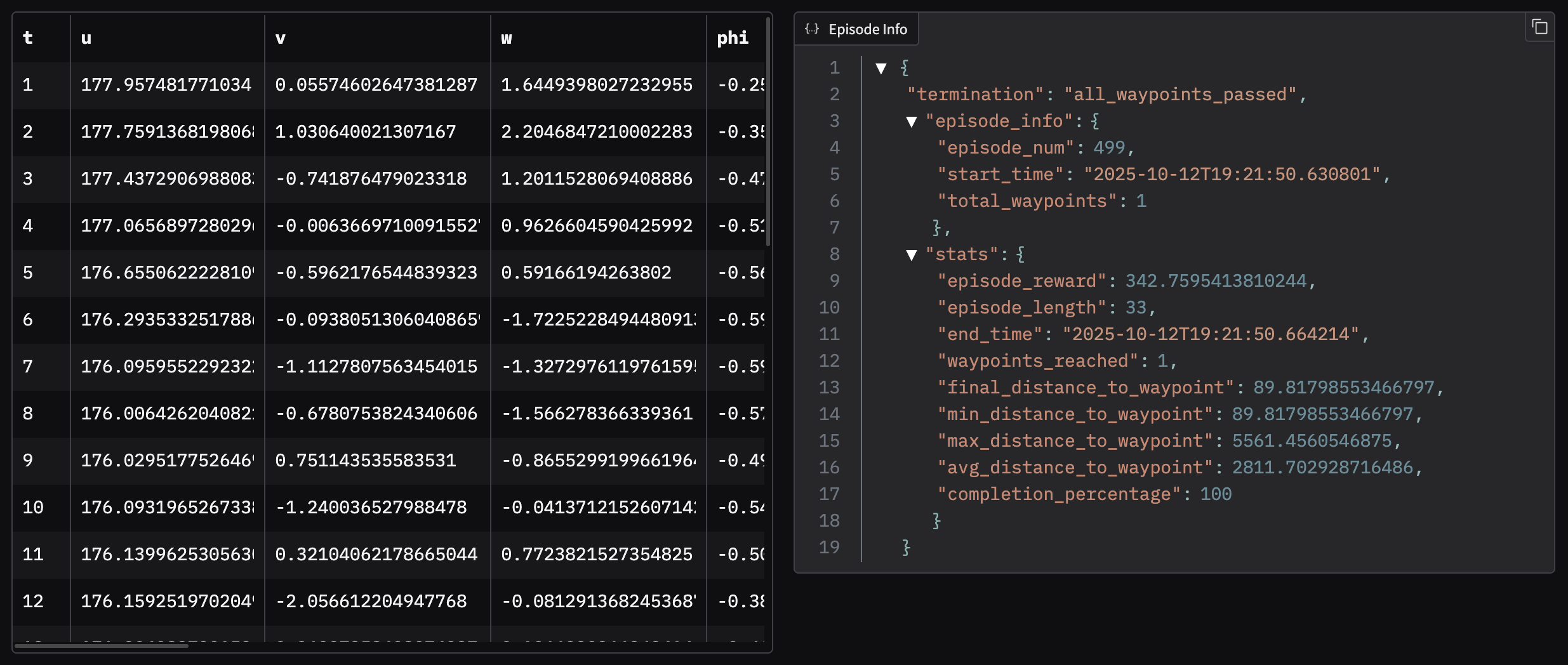
During training, the environment saves logs of the state, action, and navigation information every n episodes defined in the train config file training/configs/train_config.yaml. The logs are saved as pickle files in the training/waypoint/logs directory and can be used for later analysis or visualization. The logs include information such as the aircraft state, action taken, navigation information (such as distance to waypoint, heading error, pitch error, etc.), and reward received as well as some stats such as episode length, total reward, and number of waypoints reached. The logs can be used to analyze the agent’s performance and behavior during training or later evaluation.

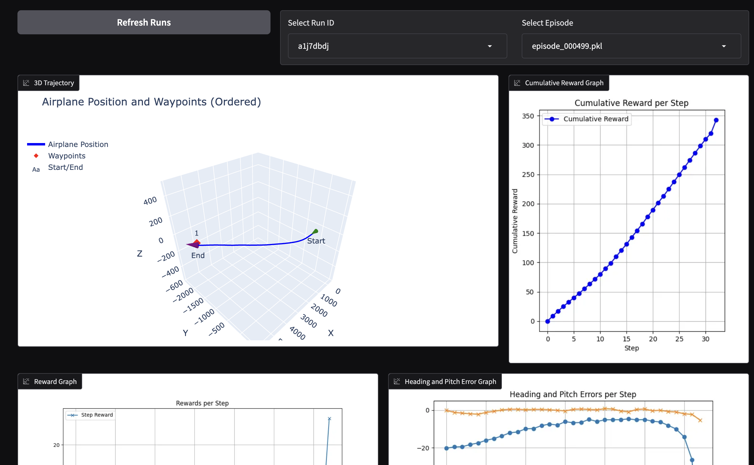
In order to facilitate the analysis of the logs, a visualization script is provided in training/waypoint/logs_visualizer.py. This script uses the Gradio library to create a simple web interface that allows loading and visualizing the logs. The script plots the 3D trajectory of the aircraft, the Euler angles and actions over time, displays the states data in a table, and other information for analysis. An example of the web interface can be seen below:

Hyperparameter Tuning

The training script uses a set of hyperparameters defined in the training/configs/train_config.yaml file. These hyperparameters include:

• Core PPO training parameters that defines how it collects experience. This includes n_stepswhich define the number of steps to run for each environment per update, batch_size which defines the minibatch size and n_epochs which defines the number of epochs to perform for each update. This parameters are important for the stability of the training and the quality of the learned policy.
• Discounting and Advantage estimation parameters that defines how future rewards are discounted and how the advantage is estimated. This includes gamma which is the discount factor from the cumulative expected reward $R_t = \sum_{k=0}^{\infty} \gamma^k r_{t+k}$, and gae_lambda which is the GAE (Generalized Advantage Estimation) parameter. These parameters are important for the trade-off between bias and variance in the value function estimation.
• Loss Function coefficients such as ent_coef which is the entropy coefficient that penalize low entropy (deterministic) policy or vf_coef which is the value function coefficient. This determines the relative importance of the value function loss compared to the policy loss.
• Policy architecture parameters such as net_arch which defines the architecture of the neural network used for the policy and value function. This includes the number of layers and the number of neurons per layer. The architecture of the neural network is important for the capacity of the model to learn complex policies. In addition, the activation function can be defined using activation_fn parameter. Since a proper initialization of the weights is important for the convergence of the training, the ortho_init parameter can be set to use orthogonal initialization for the weights of the neural network and log_std_init can be set to define the initial log standard deviation of the policy’s gaussian distribution where a lower value results in a less initial exploration.
• State dependent exploration can be enabled using the sde parameter. This allows the agent to explore more in states where it is less certain about the value function. The sde_sample_freq parameter defines how often to sample a new noise matrix for the exploration.

In order to find the best hyperparameters for the training, a hyperparameter tuning script is provided in training/waypoint/hyperparameter_search.py. This script uses the Optuna library to perform a hyperparameter search using a defined search space. The search space includes the main hyperparameters mentioned above and can be adjusted to include or exclude certain parameters. The script runs multiple trials with different hyperparameter combinations and evaluates the performance of the agent using a defined metric such as the average reward over a certain number of episodes. The results are saved to hyperparameter_search/results including the best hyperparameters found during the search.

Training and testing

To train the RL agent after setting up the agent hyperparameters and other training parameters such as total time steps, evaluation frequency, logging frequency and save paths in the training/configs/train_config.yaml file, the next step is to run the file training/waypoint/train_waypoint_control.py which loads the configuration file, creates the environment and the PPO agent, and starts the training process. The training can be run using the following command:

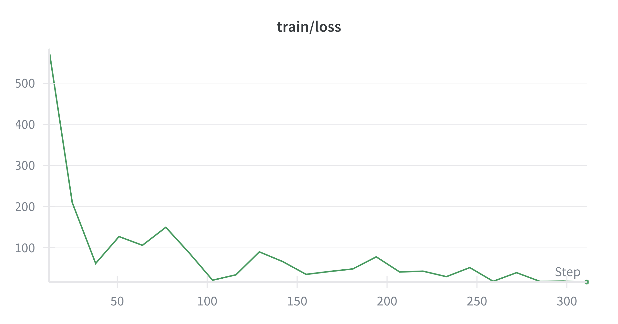
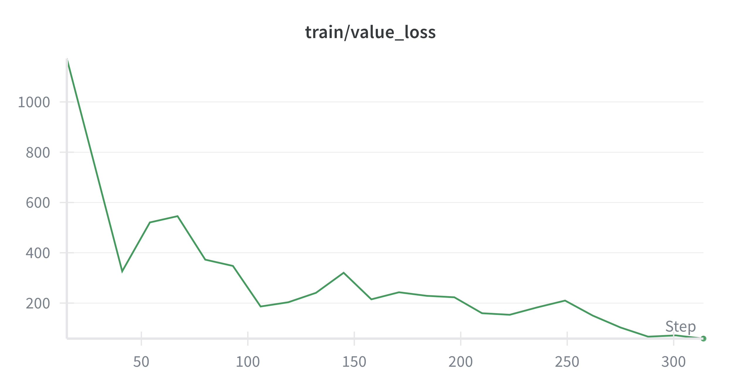
python training/waypoint/train_waypoint_control.py

The training process was devided in stages. First, the agent was trained to reach a single waypoint placed setting the minimum and maximum waypoint number to 1 in training/configs/train_config.yaml file. This allows the agent to learn the basic control of the aircraft and how to reach a waypoint. The following plots show the training loss and value loss during the training with a single waypoint. As a result of the progress defined in the reward function, the training loss decreases in few episodes and the agent is able to reach the waypoint consistently after around 100,000 time steps.

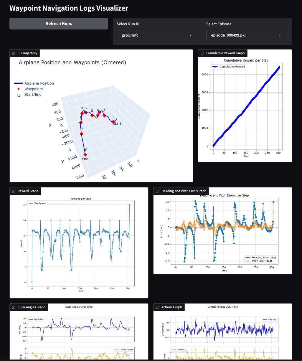
Once the agent was able to reach a single waypoint consistently, the training was continued with multiple waypoints by setting the minimum and maximum waypoint number to a higher value. This allows the agent to learn how to navigate through multiple waypoints and how to handle turns and changes in altitude. The training for just 2 waypoints is also fast and the agent is able to reach both waypoints consistently after around 500,000 time steps. For larger number of waypoints, an issue was found where the agent reach the roll limit in the transition of some waypoints. As a workaround, a higher negative reward for high roll angles was implemented to encourage the agent to avoid high roll angles. This way, the agent was able to learn to avoid high roll angles and reach all waypoints consistently after 1 million of time steps. The following plots shows the trayectory, reward, errors, euler angles and control surface deflections of an episode with 10 waypoints after training for 1 million time steps:

For testing the agent behavior visually another simple API REST is implemented in tests/agent_api which implements the same endpoints as the simulator API but instead of receiving control surface deflections, it first runs a full episode using the trained agent and then returns the state at each step. This way, the web-app can be used to visualize the agent behavior in the same way as with the simulator. To run the agent API, use the following command:

# Python API REST
cd tests
python agent_api.py

# In another terminal, run the web-app
cd simulator_webapp
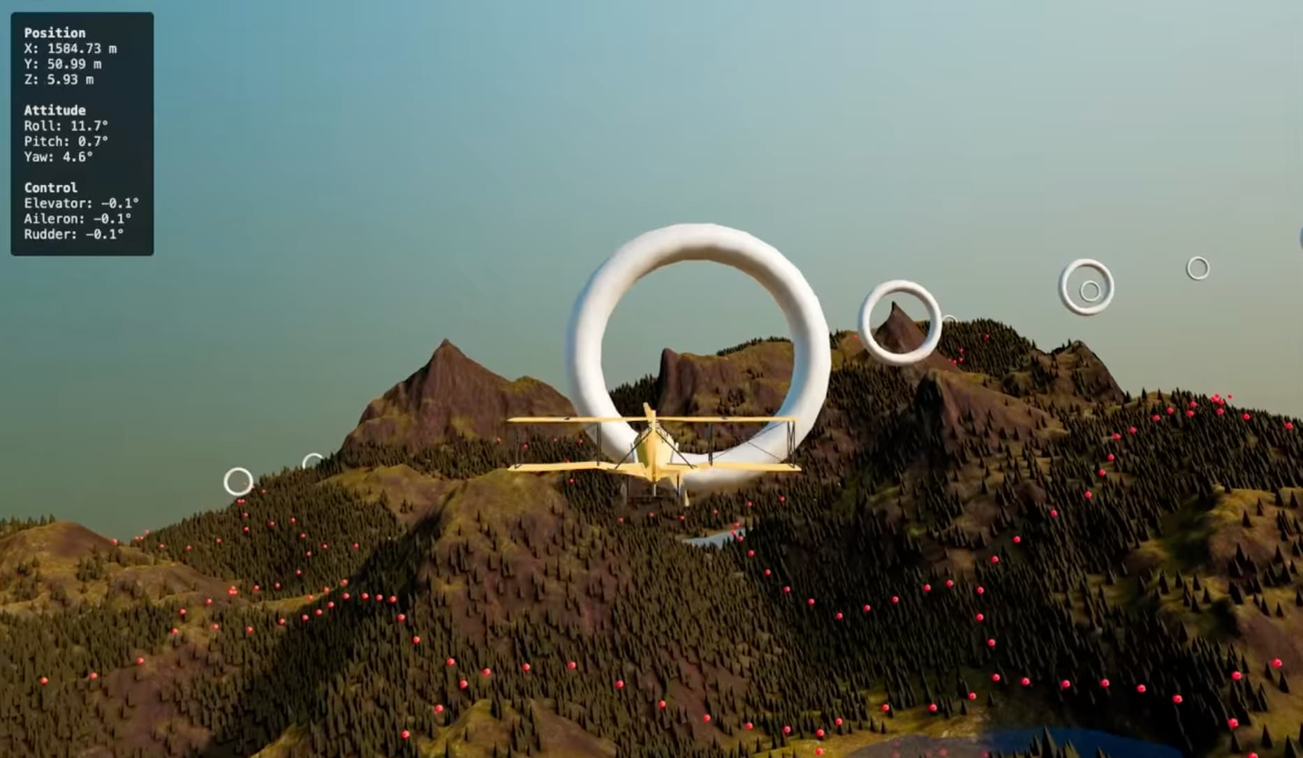
npm run dev

An example of the web-app showing the agent behavior can be seen in the video below:

where the waypoints are shown as white toruses and the aircraft is following the waypoints using smooth banking maneuvers. Despite trained to follow 10 waypoints is able to successfully follow 15 waypoints in this case. In the webapp simulator the aircraft translation is scaled for better visualization as can be seen in the state display in the upper left corner.

Acknowledgements

• [1] Miguel A. Gómez Tierno, Manuel Pérez Cortés, César Puentes Márquez, “Mecánica del Vuelo”, 2nd Edition, 2012.
• [2] Erwin Kreyszig, “Advanced Engineering Mathematics”, 10th Edition, 2011.
• [3] Francisco Giral, Ignacio Gómez, Soledad Le Clainche, “Intercepting Unauthorized Aerial Robots in Controlled Airspace Using Reinforcement Learning”, 2025.
• [4] Francisco Giral, https://github.com/fgiral000/bicopter_RL_control/tree/main, 2023.
• [5] R3F-takes-flight, https://github.com/Domenicobrz/R3F-takes-flight, 2023.
• [6] Jan Roskam, “Airplane Flight Dynamics and Automatic Flight Controls”, 2001.